Checking the spatio-temporal build up of the largest simulated events
In this notebook we will compare the UNSEEN data to the observations.
##Load pacakages
import xarray as xr
import matplotlib.pyplot as plt
import numpy as np
import cartopy
import cartopy.crs as ccrs
import pandas as pd
import calendar
##This is so variables get printed within jupyter
from IPython.core.interactiveshell import InteractiveShell
InteractiveShell.ast_node_interactivity = "all"
### Load Data
dirname = r'/home/tike/'
Observed
Observations_pooled_monthly = xr.open_dataarray('../Data/Observations_pooled_monthly.nc')
Observations_pooled_monthly
- index: 360
- 9.682e+04 1.107e+05 1.258e+05 ... 2.177e+05 1.826e+05 1.214e+05
array([ 96820.165677, 110682.521733, 125771.958613, ..., 217669.384226, 182610.150774, 121367.412367]) - index(index)datetime64[ns]1980-10-31 ... 2010-09-30
array(['1980-10-31T00:00:00.000000000', '1980-11-30T00:00:00.000000000',
       '1980-12-31T00:00:00.000000000', ..., '2010-07-31T00:00:00.000000000',
       '2010-08-31T00:00:00.000000000', '2010-09-30T00:00:00.000000000'],
      dtype='datetime64[ns]')
UNSEEN
Amazon_simulated = xr.open_dataset(dirname + 'Discharge/discharge_monthAvg_presentDay.nc')  #The data from Niko
Amazon_simulated  #to show

Amazon = Amazon_simulated['discharge'].sel(lon=-51.75, lat=-1.25)  ## Select the timeseries in the gridcell at the mouth of the river
Obidos = Amazon_simulated['discharge'].sel(lon=-55.75,lat=-2.25)  ## At the most downstream station of the main Amazon river at Obidos
Tapajos = Amazon_simulated['discharge'].sel(lon=-55.25, lat=-2.75) ## At the mouth of the southern tributary Tapajos
Xingu = Amazon_simulated['discharge'].sel(lon=-52.25, lat=-1.75)   ## Select the timeseries in the gridcell at the mouth of the river
/home/tike/miniconda3/envs/exp/lib/python3.8/site-packages/xarray/coding/times.py:426: SerializationWarning: Unable to decode time axis into full numpy.datetime64 objects, continuing using cftime.datetime objects instead, reason: dates out of range
  dtype = _decode_cf_datetime_dtype(data, units, calendar, self.use_cftime)
/home/tike/miniconda3/envs/exp/lib/python3.8/site-packages/numpy/core/_asarray.py:85: SerializationWarning: Unable to decode time axis into full numpy.datetime64 objects, continuing using cftime.datetime objects instead, reason: dates out of range
  return array(a, dtype, copy=False, order=order)
- lat: 44
- lon: 70
- time: 24000
- time(time)object0001-01-03 00:00:00 ... 2055-01-01 00:00:00
- standard_name :
- time
- long_name :
- Days since 1901-01-01
array([cftime.DatetimeGregorian(0001-01-03 00:00:00), cftime.DatetimeGregorian(0002-01-03 00:00:00), cftime.DatetimeGregorian(0003-01-03 00:00:00), ..., cftime.DatetimeGregorian(2053-01-01 00:00:00), cftime.DatetimeGregorian(2054-01-01 00:00:00), cftime.DatetimeGregorian(2055-01-01 00:00:00)], dtype=object) - lat(lat)float324.75 4.25 3.75 ... -16.25 -16.75
- long_name :
- latitude
- units :
- degrees_north
- standard_name :
- latitude
array([ 4.75, 4.25, 3.75, 3.25, 2.75, 2.25, 1.75, 1.25, 0.75, 0.25, -0.25, -0.75, -1.25, -1.75, -2.25, -2.75, -3.25, -3.75, -4.25, -4.75, -5.25, -5.75, -6.25, -6.75, -7.25, -7.75, -8.25, -8.75, -9.25, -9.75, -10.25, -10.75, -11.25, -11.75, -12.25, -12.75, -13.25, -13.75, -14.25, -14.75, -15.25, -15.75, -16.25, -16.75], dtype=float32) - lon(lon)float32-79.75 -79.25 ... -45.75 -45.25
- standard_name :
- longitude
- long_name :
- longitude
- units :
- degrees_east
array([-79.75, -79.25, -78.75, -78.25, -77.75, -77.25, -76.75, -76.25, -75.75,
       -75.25, -74.75, -74.25, -73.75, -73.25, -72.75, -72.25, -71.75, -71.25,
       -70.75, -70.25, -69.75, -69.25, -68.75, -68.25, -67.75, -67.25, -66.75,
       -66.25, -65.75, -65.25, -64.75, -64.25, -63.75, -63.25, -62.75, -62.25,
       -61.75, -61.25, -60.75, -60.25, -59.75, -59.25, -58.75, -58.25, -57.75,
       -57.25, -56.75, -56.25, -55.75, -55.25, -54.75, -54.25, -53.75, -53.25,
       -52.75, -52.25, -51.75, -51.25, -50.75, -50.25, -49.75, -49.25, -48.75,
       -48.25, -47.75, -47.25, -46.75, -46.25, -45.75, -45.25], dtype=float32)
- discharge(time, lat, lon)float32...
- standard_name :
- discharge
- long_name :
- discharge
- units :
- m3s-1
[73920000 values with dtype=float32]
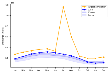
The temporal characteristics of the floods
Now we will compare the flood seasonality between UNSEEN simulations and the observations. We plot the 2, 20 and 2000 year monthly flood values for UNSEEN and the 2, 20 and 52 year values for the observations.
The plot shows that there are large UNSEEN floods in July-September, that are not seen in the observations.
##Create a time array for indexing the time dimension
#The time axis is currently from 0:2000, I will change them to their original years 2035-2040 (copied from the precipitation dataset).
# The runs are five years long, repeated 400 times (16 starts x 25 ensembles).
# Time_year represents one run, that should be repeated 400 times to match the time dimension.
time_year=np.arange('2035-01', '2040-01', dtype='datetime64[M]')
time_year
array(['2035-01', '2035-02', '2035-03', '2035-04', '2035-05', '2035-06',
       '2035-07', '2035-08', '2035-09', '2035-10', '2035-11', '2035-12',
       '2036-01', '2036-02', '2036-03', '2036-04', '2036-05', '2036-06',
       '2036-07', '2036-08', '2036-09', '2036-10', '2036-11', '2036-12',
       '2037-01', '2037-02', '2037-03', '2037-04', '2037-05', '2037-06',
       '2037-07', '2037-08', '2037-09', '2037-10', '2037-11', '2037-12',
       '2038-01', '2038-02', '2038-03', '2038-04', '2038-05', '2038-06',
       '2038-07', '2038-08', '2038-09', '2038-10', '2038-11', '2038-12',
       '2039-01', '2039-02', '2039-03', '2039-04', '2039-05', '2039-06',
       '2039-07', '2039-08', '2039-09', '2039-10', '2039-11', '2039-12'],
      dtype='datetime64[M]')
### Set extent and projection
plt.rcParams["font.family"] = "sans-serif" ##change font
plt.rcParams['font.size'] = 7  ## change font size (6 was used below)
plt.rcParams['svg.fonttype'] = 'none' ## so inkscape recognized texts in svg file
plt.rcParams['pdf.fonttype'] = 42 ## so illustrator can recognize text
# plt.figure(figsize=(90/25.4, 40/25.4))
ax = plt.axes()
Quantiles_obs = Observations_pooled_monthly.groupby("index.month").quantile([0,1-1/2, 1-1/20, 1], dim="index")
ax.fill_between(list(calendar.month_abbr[1:]), Quantiles_obs.sel(quantile=1-1/2), Quantiles_obs.sel(quantile=1-1/20), color='blue', alpha=0.2,label = '20-year')
ax.fill_between(list(calendar.month_abbr[1:]), Quantiles_obs.sel(quantile=0), Quantiles_obs.sel(quantile=1-1/2), color='blue', alpha=0.1,label = '2-year')

plt.plot(list(calendar.month_abbr[1:]),
         Amazon.assign_coords(
             time=np.tile(time_year, 400)).isel(
             time=slice(1567 * 12, 1568 * 12)
         ).values,
         marker='o',
         markersize = 4,
         label='largest simulation',
         color='orange'
        )

plt.plot(list(calendar.month_abbr[1:]),
         Observations_pooled_monthly.sel(
             index=slice('2009', '2009-12')
         ).values,
         marker='o',
         markersize = 4,
         label='2009',
         color='blue'
        )

plt.ylabel('Discharge [m3/s]')
plt.legend()
# plt.savefig('../Graphs/paper/Discharge_temporal_obs_flood1.pdf',bbox_inches='tight', dpi =300)
<matplotlib.collections.PolyCollection at 0x2ad54d9e1e20>
<matplotlib.collections.PolyCollection at 0x2ad54d9e8580>
[<matplotlib.lines.Line2D at 0x2ad54d9e1e80>]
[<matplotlib.lines.Line2D at 0x2ad54d9fb070>]
Text(0, 0.5, 'Discharge [m3/s]')
<matplotlib.legend.Legend at 0x2ad54d9e8e80>
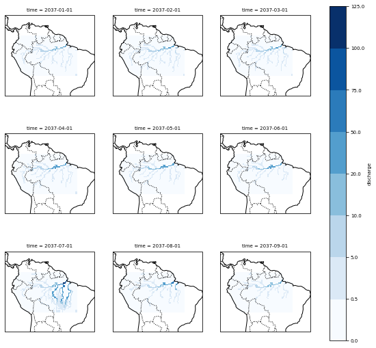
The spatial characteristics
For the spatial characteristics, we first plot the streamflow for the entire basin in % of the flood, for each month of the year preceding the flood. The index for the flood is selected here.
##Flood1
Amazon_discharge_all_months_flood1 = Amazon_simulated.assign_coords(time=np.tile(time_year,400)).isel(time=slice(1566*12,1568*12))
Amazon_discharge_all_months_flood1_normalized_toflood = Amazon_discharge_all_months_flood1/ Amazon_discharge_all_months_flood1.sel(time='2037-07-01',lon=-51.75, lat=-1.25) *100
Amazon_discharge_all_months_flood1.sel(time='2037-07-01',lon=-51.75, lat=-1.25)
Amazon_discharge_all_months_flood1
- time()datetime64[ns]2037-07-01
array('2037-07-01T00:00:00.000000000', dtype='datetime64[ns]') - lat()float32-1.25
- long_name :
- latitude
- units :
- degrees_north
- standard_name :
- latitude
array(-1.25, dtype=float32)
- lon()float32-51.75
- standard_name :
- longitude
- long_name :
- longitude
- units :
- degrees_east
array(-51.75, dtype=float32)
- discharge()float32...
- standard_name :
- discharge
- long_name :
- discharge
- units :
- m3s-1
array(1157535.75)
- lat: 44
- lon: 70
- time: 24
- time(time)datetime64[ns]2036-01-01 ... 2037-12-01
array(['2036-01-01T00:00:00.000000000', '2036-02-01T00:00:00.000000000', '2036-03-01T00:00:00.000000000', '2036-04-01T00:00:00.000000000', '2036-05-01T00:00:00.000000000', '2036-06-01T00:00:00.000000000', '2036-07-01T00:00:00.000000000', '2036-08-01T00:00:00.000000000', '2036-09-01T00:00:00.000000000', '2036-10-01T00:00:00.000000000', '2036-11-01T00:00:00.000000000', '2036-12-01T00:00:00.000000000', '2037-01-01T00:00:00.000000000', '2037-02-01T00:00:00.000000000', '2037-03-01T00:00:00.000000000', '2037-04-01T00:00:00.000000000', '2037-05-01T00:00:00.000000000', '2037-06-01T00:00:00.000000000', '2037-07-01T00:00:00.000000000', '2037-08-01T00:00:00.000000000', '2037-09-01T00:00:00.000000000', '2037-10-01T00:00:00.000000000', '2037-11-01T00:00:00.000000000', '2037-12-01T00:00:00.000000000'], dtype='datetime64[ns]') - lat(lat)float324.75 4.25 3.75 ... -16.25 -16.75
- long_name :
- latitude
- units :
- degrees_north
- standard_name :
- latitude
array([ 4.75, 4.25, 3.75, 3.25, 2.75, 2.25, 1.75, 1.25, 0.75, 0.25, -0.25, -0.75, -1.25, -1.75, -2.25, -2.75, -3.25, -3.75, -4.25, -4.75, -5.25, -5.75, -6.25, -6.75, -7.25, -7.75, -8.25, -8.75, -9.25, -9.75, -10.25, -10.75, -11.25, -11.75, -12.25, -12.75, -13.25, -13.75, -14.25, -14.75, -15.25, -15.75, -16.25, -16.75], dtype=float32) - lon(lon)float32-79.75 -79.25 ... -45.75 -45.25
- standard_name :
- longitude
- long_name :
- longitude
- units :
- degrees_east
array([-79.75, -79.25, -78.75, -78.25, -77.75, -77.25, -76.75, -76.25, -75.75,
       -75.25, -74.75, -74.25, -73.75, -73.25, -72.75, -72.25, -71.75, -71.25,
       -70.75, -70.25, -69.75, -69.25, -68.75, -68.25, -67.75, -67.25, -66.75,
       -66.25, -65.75, -65.25, -64.75, -64.25, -63.75, -63.25, -62.75, -62.25,
       -61.75, -61.25, -60.75, -60.25, -59.75, -59.25, -58.75, -58.25, -57.75,
       -57.25, -56.75, -56.25, -55.75, -55.25, -54.75, -54.25, -53.75, -53.25,
       -52.75, -52.25, -51.75, -51.25, -50.75, -50.25, -49.75, -49.25, -48.75,
       -48.25, -47.75, -47.25, -46.75, -46.25, -45.75, -45.25], dtype=float32)
- discharge(time, lat, lon)float32...
- standard_name :
- discharge
- long_name :
- discharge
- units :
- m3s-1
array([[[        nan,         nan, ...,         nan,         nan],
        [        nan,         nan, ...,         nan,         nan],
        ...,
        [        nan,         nan, ...,  832.3572  , 6813.952   ],
        [        nan,         nan, ...,   62.77098 , 5882.9917  ]],

       [[        nan,         nan, ...,         nan,         nan],
        [        nan,         nan, ...,         nan,         nan],
        ...,
        [        nan,         nan, ...,  650.74854 , 6527.3936  ],
        [        nan,         nan, ...,   62.75068 , 5777.773   ]],

       ...,

       [[        nan,         nan, ...,         nan,         nan],
        [        nan,         nan, ...,         nan,         nan],
        ...,
        [        nan,         nan, ...,  151.99892 , 2370.2266  ],
        [        nan,         nan, ...,   13.659762, 2191.7114  ]],

       [[        nan,         nan, ...,         nan,         nan],
        [        nan,         nan, ...,         nan,         nan],
        ...,
        [        nan,         nan, ...,  221.49239 , 3726.3708  ],
        [        nan,         nan, ...,   15.650466, 3473.6763  ]]],
      dtype=float32)
extent = [-85, -35, 15, -25]
levels = [0, 0.5, 5, 10, 20, 50, 75,100,125]
# g_simple=Amazon_discharge_all_months_flood1_normalized['discharge'].sel(time=slice('2036-11-16T12:00:00.000000000','2037-11-16T00:00:00.000000000')).plot(transform=ccrs.PlateCarree(),levels=levels,cmap=plt.cm.Blues, col='time', col_wrap=3,subplot_kws={'projection': ccrs.Mercator()})  #,cmap=plt.cm.Blues,
g_simple=Amazon_discharge_all_months_flood1_normalized_toflood['discharge'].sel(time=slice('2037-01','2037-09')).plot(transform=ccrs.PlateCarree(),cmap=plt.cm.Blues, levels=levels, col='time', col_wrap=3,subplot_kws={'projection': ccrs.Mercator()})  #,cmap=plt.cm.Blues,

for ax in g_simple.axes.flat:
    ax.set_extent(extent)
    ax.coastlines(resolution='110m')
    ax.add_feature(cartopy.feature.BORDERS, linestyle=':')
#     ax.gridlines()

plt.draw()
plt.savefig('../Graphs/Discharge_spatial_flood1.png',bbox_inches='tight',dpi =300)
<cartopy.mpl.feature_artist.FeatureArtist at 0x2ad54fec3190>
<cartopy.mpl.feature_artist.FeatureArtist at 0x2ad54fefdc40>
<cartopy.mpl.feature_artist.FeatureArtist at 0x2ad54fefdc10>
<cartopy.mpl.feature_artist.FeatureArtist at 0x2ad54fefd640>
<cartopy.mpl.feature_artist.FeatureArtist at 0x2ad54fefd7f0>
<cartopy.mpl.feature_artist.FeatureArtist at 0x2ad54fefd1f0>
<cartopy.mpl.feature_artist.FeatureArtist at 0x2ad54fef9c70>
<cartopy.mpl.feature_artist.FeatureArtist at 0x2ad54fef9d60>
<cartopy.mpl.feature_artist.FeatureArtist at 0x2ad54fb949a0>
<cartopy.mpl.feature_artist.FeatureArtist at 0x2ad54fef9c10>
<cartopy.mpl.feature_artist.FeatureArtist at 0x2ad54fef9df0>
<cartopy.mpl.feature_artist.FeatureArtist at 0x2ad54ff010a0>
<cartopy.mpl.feature_artist.FeatureArtist at 0x2ad54ff01af0>
<cartopy.mpl.feature_artist.FeatureArtist at 0x2ad54ff010d0>
<cartopy.mpl.feature_artist.FeatureArtist at 0x2ad54ff01cd0>
<cartopy.mpl.feature_artist.FeatureArtist at 0x2ad54ff019d0>
<cartopy.mpl.feature_artist.FeatureArtist at 0x2ad54ff01eb0>
<cartopy.mpl.feature_artist.FeatureArtist at 0x2ad54ff01bb0>
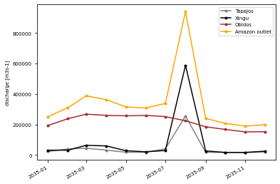
We then look at the streamflow at a few locations within the Amazon catchment during the highest streamflow simulation within the model experiments.
For the largest flood:
# plt.figure(figsize=(90/25.4, 40/25.4))

Tapajos.assign_coords(
    time=np.tile(time_year, 400)).isel(                          ## Not very neat, but here we assign the time_year, repeated 400 times.
    time=slice(1566 * 12, 1568 * 12)).plot.line(marker='o',      ## And then we can select the index of the highest flood and plot a line
                                                markersize= 3,
                                                label='Tapajos',
                                                color='grey')

Xingu.assign_coords(                                             ## Same for Xingu
    time=np.tile(time_year, 400)).isel(
    time=slice(1566 * 12, 1568 * 12)).plot.line(marker='o',
                                                markersize = 3,
                                                label='Xingu',
                                                color='black')
Obidos.assign_coords(                                             ## Same for Xingu
    time=np.tile(time_year, 400)).isel(
    time=slice(1566 * 12, 1568 * 12)).plot.line(marker='o',
                                                markersize = 3,
                                                label='Obidos',
                                                color='brown')
Amazon.assign_coords(
    time=np.tile(time_year, 400)).isel(                          ## And the Amazon mouth.
    time=slice(1566 * 12, 1568 * 12)).plot.line(marker='o',
                                                markersize = 3,
                                                label='Amazon outlet',
                                                color='orange')
plt.legend()
plt.title("")
plt.xlabel("")
plt.draw()
# plt.savefig('../Graphs/paper/Discharge_spatial_flood1.pdf',bbox_inches='tight',dpi =300)
[<matplotlib.lines.Line2D at 0x2ad54da2cfd0>]
[<matplotlib.lines.Line2D at 0x2ad54da64430>]
[<matplotlib.lines.Line2D at 0x2ad54da68460>]
[<matplotlib.lines.Line2D at 0x2ad54da68ee0>]
<matplotlib.legend.Legend at 0x2ad54da64940>
Text(0.5, 1.0, '')
Text(0.5, 0, '')
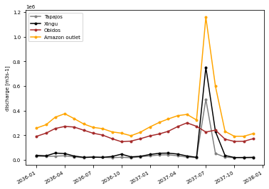
And the second largest flood:
# plt.figure(figsize=(90/25.4, 40/25.4))

Tapajos.assign_coords(
    time=np.tile(time_year, 400)).isel(                          ## Not very neat, but here we assign the time_year, repeated 400 times.
    time=slice(1730 * 12, 1731 * 12)).plot.line(marker='o',      ## And then we can select the index of the highest flood and plot a line
                                                markersize= 3,
                                                label='Tapajos',
                                                color='grey')

Xingu.assign_coords(                                             ## Same for Xingu
    time=np.tile(time_year, 400)).isel(
    time=slice(1730 * 12, 1731 * 12)).plot.line(marker='o',
                                                markersize = 3,
                                                label='Xingu',
                                                color='black')
Obidos.assign_coords(                                             ## Same for Xingu
    time=np.tile(time_year, 400)).isel(
    time=slice(1730 * 12, 1731 * 12)).plot.line(marker='o',
                                                markersize = 3,
                                                label='Obidos',
                                                color='brown')
Amazon.assign_coords(
    time=np.tile(time_year, 400)).isel(                          ## And the Amazon mouth.
    time=slice(1730 * 12, 1731 * 12)).plot.line(marker='o',
                                                markersize = 3,
                                                label='Amazon outlet',
                                                color='orange')
plt.legend()
plt.title("")
plt.xlabel("")
plt.draw()
# plt.savefig('../Graphs/paper/Discharge_spatial_flood2.png',bbox_inches='tight',dpi =300)
[<matplotlib.lines.Line2D at 0x2ad52bf13850>]
[<matplotlib.lines.Line2D at 0x2ad54dbc7970>]
[<matplotlib.lines.Line2D at 0x2ad54dbc7ee0>]
[<matplotlib.lines.Line2D at 0x2ad54dbcd580>]
<matplotlib.legend.Legend at 0x2ad54dbc7fd0>
Text(0.5, 1.0, '')
Text(0.5, 0, '')