When did the two highest mega floods in the Amazon occur?
We found two simulated mega-floods, that largely deviated from what can be expected from the observed record. Here we will perform a first analysis to figure out when they happened.
##Load pacakages
import xarray as xr
import matplotlib.pyplot as plt
import numpy as np
import cartopy
import cartopy.crs as ccrs
##This is so variables get printed within jupyter
from IPython.core.interactiveshell import InteractiveShell
InteractiveShell.ast_node_interactivity = "all"
We are loading the data from (der Wiel et al., 2019), openly available through https://zenodo.org/record/2536396#.XnnBgohKiUk.
Note the error message in regard to the time. I suspect this is because it is just a number from 1:2000 -> there are 2000 present-climate and future-climate years.
UNSEEN floods
Load the simulations (discharge_monthAvg_presentDay.nc) available at https://doi.org/10.5281/zenodo.4585400 or download them in the ../Data directory by uncommenting and running the following line:
!wget -O ../Data/discharge_monthAvg_presentDay.nc https://zenodo.org/record/4585400/files/discharge_monthAvg_presentDay.nc
--2021-10-07 13:09:36--  https://zenodo.org/record/4585400/files/discharge_monthAvg_presentDay.nc
Resolving zenodo.org (zenodo.org)... 137.138.76.77
Connecting to zenodo.org (zenodo.org)|137.138.76.77|:443... connected.
HTTP request sent, awaiting response... 200 OK
Length: 247755472 (236M) [application/octet-stream]
Saving to: ‘../Data/discharge_monthAvg_presentDay.nc’

100%[======================================>] 247,755,472 40.7MB/s   in 5.8s

2021-10-07 13:09:42 (40.7 MB/s) - ‘../Data/discharge_monthAvg_presentDay.nc’ saved [247755472/247755472]
Amazon_simulated = xr.open_dataset('../Data/discharge_monthAvg_presentDay.nc')
Amazon_simulated #to show
/home/tike/miniconda3/envs/exp/lib/python3.8/site-packages/xarray/coding/times.py:426: SerializationWarning: Unable to decode time axis into full numpy.datetime64 objects, continuing using cftime.datetime objects instead, reason: dates out of range
  dtype = _decode_cf_datetime_dtype(data, units, calendar, self.use_cftime)
/home/tike/miniconda3/envs/exp/lib/python3.8/site-packages/numpy/core/_asarray.py:85: SerializationWarning: Unable to decode time axis into full numpy.datetime64 objects, continuing using cftime.datetime objects instead, reason: dates out of range
  return array(a, dtype, copy=False, order=order)
- lat: 44
- lon: 70
- time: 24000
- time(time)object0001-01-03 00:00:00 ... 2055-01-01 00:00:00
- standard_name :
- time
- long_name :
- Days since 1901-01-01
array([cftime.DatetimeGregorian(0001-01-03 00:00:00), cftime.DatetimeGregorian(0002-01-03 00:00:00), cftime.DatetimeGregorian(0003-01-03 00:00:00), ..., cftime.DatetimeGregorian(2053-01-01 00:00:00), cftime.DatetimeGregorian(2054-01-01 00:00:00), cftime.DatetimeGregorian(2055-01-01 00:00:00)], dtype=object) - lat(lat)float324.75 4.25 3.75 ... -16.25 -16.75
- long_name :
- latitude
- units :
- degrees_north
- standard_name :
- latitude
array([ 4.75, 4.25, 3.75, 3.25, 2.75, 2.25, 1.75, 1.25, 0.75, 0.25, -0.25, -0.75, -1.25, -1.75, -2.25, -2.75, -3.25, -3.75, -4.25, -4.75, -5.25, -5.75, -6.25, -6.75, -7.25, -7.75, -8.25, -8.75, -9.25, -9.75, -10.25, -10.75, -11.25, -11.75, -12.25, -12.75, -13.25, -13.75, -14.25, -14.75, -15.25, -15.75, -16.25, -16.75], dtype=float32) - lon(lon)float32-79.75 -79.25 ... -45.75 -45.25
- standard_name :
- longitude
- long_name :
- longitude
- units :
- degrees_east
array([-79.75, -79.25, -78.75, -78.25, -77.75, -77.25, -76.75, -76.25, -75.75,
       -75.25, -74.75, -74.25, -73.75, -73.25, -72.75, -72.25, -71.75, -71.25,
       -70.75, -70.25, -69.75, -69.25, -68.75, -68.25, -67.75, -67.25, -66.75,
       -66.25, -65.75, -65.25, -64.75, -64.25, -63.75, -63.25, -62.75, -62.25,
       -61.75, -61.25, -60.75, -60.25, -59.75, -59.25, -58.75, -58.25, -57.75,
       -57.25, -56.75, -56.25, -55.75, -55.25, -54.75, -54.25, -53.75, -53.25,
       -52.75, -52.25, -51.75, -51.25, -50.75, -50.25, -49.75, -49.25, -48.75,
       -48.25, -47.75, -47.25, -46.75, -46.25, -45.75, -45.25], dtype=float32)
- discharge(time, lat, lon)float32...
- standard_name :
- discharge
- long_name :
- discharge
- units :
- m3s-1
[73920000 values with dtype=float32]
dirname = r'/home/tike/Discharge/'

Global_discharge = xr.open_dataset(dirname + 'Zenodo/presentYearMax.nc')
Global_discharge
/home/tike/miniconda3/envs/exp/lib/python3.8/site-packages/xarray/coding/times.py:426: SerializationWarning: Unable to decode time axis into full numpy.datetime64 objects, continuing using cftime.datetime objects instead, reason: dates out of range
  dtype = _decode_cf_datetime_dtype(data, units, calendar, self.use_cftime)
/home/tike/miniconda3/envs/exp/lib/python3.8/site-packages/numpy/core/_asarray.py:85: SerializationWarning: Unable to decode time axis into full numpy.datetime64 objects, continuing using cftime.datetime objects instead, reason: dates out of range
  return array(a, dtype, copy=False, order=order)
- lat: 360
- lon: 720
- time: 2000
- time(time)object0001-01-01 00:00:00 ... 2000-01-01 00:00:00
- standard_name :
- time
- long_name :
- Days since 1901-01-01
array([cftime.DatetimeGregorian(0001-01-01 00:00:00), cftime.DatetimeGregorian(0002-01-01 00:00:00), cftime.DatetimeGregorian(0003-01-01 00:00:00), ..., cftime.DatetimeGregorian(1998-01-01 00:00:00), cftime.DatetimeGregorian(1999-01-01 00:00:00), cftime.DatetimeGregorian(2000-01-01 00:00:00)], dtype=object) - lat(lat)float3289.75 89.25 88.75 ... -89.25 -89.75
- long_name :
- latitude
- units :
- degrees_north
- standard_name :
- latitude
array([ 89.75, 89.25, 88.75, ..., -88.75, -89.25, -89.75], dtype=float32)
- lon(lon)float32-179.75 -179.25 ... 179.25 179.75
- standard_name :
- longitude
- long_name :
- longitude
- units :
- degrees_east
array([-179.75, -179.25, -178.75, ...,  178.75,  179.25,  179.75],
      dtype=float32)
- discharge(time, lat, lon)float32...
- standard_name :
- discharge
- long_name :
- discharge
- units :
- m3s-1
[518400000 values with dtype=float32]
Selecting the streamflow timeseries for the mouth of the Amazon
The files contain 2000 years of annual monthly maximum streamflow. So far I have used the mouth of the river by selecting the gridcell with the highest streamflow.
Todo
[] Change the location to Obidos for comparison to observed?
##Spatial domain of the Amazon basin
lats = [5, -17]
lons = [-80, -45]

## We cut out the Amazon region
Amazon_discharge = Global_discharge['discharge'].sel(lon=slice(lons[0], lons[1]),
                                           lat=slice(lats[0], lats[1]))
Amazon_discharge
- time: 2000
- lat: 44
- lon: 70
- ...
[6160000 values with dtype=float32]
- time(time)object0001-01-01 00:00:00 ... 2000-01-01 00:00:00
- standard_name :
- time
- long_name :
- Days since 1901-01-01
array([cftime.DatetimeGregorian(0001-01-01 00:00:00), cftime.DatetimeGregorian(0002-01-01 00:00:00), cftime.DatetimeGregorian(0003-01-01 00:00:00), ..., cftime.DatetimeGregorian(1998-01-01 00:00:00), cftime.DatetimeGregorian(1999-01-01 00:00:00), cftime.DatetimeGregorian(2000-01-01 00:00:00)], dtype=object) - lat(lat)float324.75 4.25 3.75 ... -16.25 -16.75
- long_name :
- latitude
- units :
- degrees_north
- standard_name :
- latitude
array([ 4.75, 4.25, 3.75, 3.25, 2.75, 2.25, 1.75, 1.25, 0.75, 0.25, -0.25, -0.75, -1.25, -1.75, -2.25, -2.75, -3.25, -3.75, -4.25, -4.75, -5.25, -5.75, -6.25, -6.75, -7.25, -7.75, -8.25, -8.75, -9.25, -9.75, -10.25, -10.75, -11.25, -11.75, -12.25, -12.75, -13.25, -13.75, -14.25, -14.75, -15.25, -15.75, -16.25, -16.75], dtype=float32) - lon(lon)float32-79.75 -79.25 ... -45.75 -45.25
- standard_name :
- longitude
- long_name :
- longitude
- units :
- degrees_east
array([-79.75, -79.25, -78.75, -78.25, -77.75, -77.25, -76.75, -76.25, -75.75,
       -75.25, -74.75, -74.25, -73.75, -73.25, -72.75, -72.25, -71.75, -71.25,
       -70.75, -70.25, -69.75, -69.25, -68.75, -68.25, -67.75, -67.25, -66.75,
       -66.25, -65.75, -65.25, -64.75, -64.25, -63.75, -63.25, -62.75, -62.25,
       -61.75, -61.25, -60.75, -60.25, -59.75, -59.25, -58.75, -58.25, -57.75,
       -57.25, -56.75, -56.25, -55.75, -55.25, -54.75, -54.25, -53.75, -53.25,
       -52.75, -52.25, -51.75, -51.25, -50.75, -50.25, -49.75, -49.25, -48.75,
       -48.25, -47.75, -47.25, -46.75, -46.25, -45.75, -45.25], dtype=float32)
- standard_name :
- discharge
- long_name :
- discharge
- units :
- m3s-1
### Select amazon timeseries -> 1 select the highest mean discharge over the domain (which is at the mouth of the river)
Gridpoint_Highest_mean = Amazon_discharge.mean(dim=['time']).max(
    dim=['lon', 'lat'])
Gridpoint_Highest_mean
/home/tike/miniconda3/envs/exp/lib/python3.8/site-packages/xarray/core/nanops.py:142: RuntimeWarning: Mean of empty slice
  return np.nanmean(a, axis=axis, dtype=dtype)
- 349802.16
array(349802.16, dtype=float32)
## Select amazon timeseries -> 2. extract the corresponding grid cell with the highest discharge
Amazon_timeseries = Amazon_discharge.where(
    Amazon_discharge.mean(dim=['time']) == Gridpoint_Highest_mean, drop=True)

Amazon_timeseries
- time: 2000
- lat: 1
- lon: 1
- 288759.75 315094.16 358959.7 ... 406101.53 389518.06 355163.88
array([[[288759.75]], [[315094.16]], [[358959.7 ]], ..., [[406101.53]], [[389518.06]], [[355163.88]]], dtype=float32) - time(time)object0001-01-01 00:00:00 ... 2000-01-01 00:00:00
- standard_name :
- time
- long_name :
- Days since 1901-01-01
array([cftime.DatetimeGregorian(0001-01-01 00:00:00), cftime.DatetimeGregorian(0002-01-01 00:00:00), cftime.DatetimeGregorian(0003-01-01 00:00:00), ..., cftime.DatetimeGregorian(1998-01-01 00:00:00), cftime.DatetimeGregorian(1999-01-01 00:00:00), cftime.DatetimeGregorian(2000-01-01 00:00:00)], dtype=object) - lat(lat)float320.25
- long_name :
- latitude
- units :
- degrees_north
- standard_name :
- latitude
array([0.25], dtype=float32)
- lon(lon)float32-50.25
- standard_name :
- longitude
- long_name :
- longitude
- units :
- degrees_east
array([-50.25], dtype=float32)
- standard_name :
- discharge
- long_name :
- discharge
- units :
- m3s-1
##lat 0.25
##lon -50.25

## Alternative: select with latlon
Amazon_timeseries_p = Global_discharge['discharge'].sel(lon=-50.25,
                                             lat=0.25)  ## just to check
# Amazon_timeseries_f = xr_f['discharge'].sel(lon=-50.25,
#                                             lat=0.25)  # And select future

# And save to be used in R
#np.savetxt(dirname+'presentYearMax_Amazon.txt',Amazon_timeseries_p.values.flatten())
#np.savetxt(dirname+'futureYearMax_Amazon.txt',Amazon_timeseries_f.values.flatten())
Mega-flood indices
We have now selected the timeseries for the mouth of the Amazon. Next step is to extract the two highest events, that are deviating a lot from the rest (see Extreme value analysis.
The highest flood occurs on 1568 (index 1567 in python). The second highest on 1731 (index 1730 in python).
For megaflood1 this corresponds to: Year: 2037 Start: 13 Ensemble: 13
And for megaflood2 this corresponds to: Year: 2035 Start: 14 Ensemble: 21
After we found the bias correction error: the higest MAM flood occurs on 1292.
# List from Niko:
# S01-E01-2035 S01-E01-2036 S01-E01-2037 S01-E01-2038 S01-E01-2039 S01 E02 -2035…. S01-E16-2039 S02-E01-2035…

Starts=np.arange(1,17)
Ensembles=np.arange(0,25)
years=np.arange(2035,2040)
Starts
Ensembles
years
array([ 1, 2, 3, 4, 5, 6, 7, 8, 9, 10, 11, 12, 13, 14, 15, 16])
array([ 0,  1,  2,  3,  4,  5,  6,  7,  8,  9, 10, 11, 12, 13, 14, 15, 16,
       17, 18, 19, 20, 21, 22, 23, 24])
array([2035, 2036, 2037, 2038, 2039])
years_list=np.tile(years,len(Starts)*len(Ensembles))
Starts_list=np.array([])
for start in Starts:
    Starts_list = np.append(Starts_list, np.repeat(start,len(years)*len(Ensembles)))
Ensembles_list_signlestart=np.array([])
for ensemble in Ensembles:
    Ensembles_list_signlestart = np.append(Ensembles_list_signlestart, np.repeat(ensemble,len(years)))
Ensembles_list=np.tile(Ensembles_list_signlestart,len(Starts))
years_list[0:200]
Ensembles_list[0:200]
Starts_list[0:200]

len(years_list)
len(Starts_list)
len(Ensembles_list)
array([2035, 2036, 2037, 2038, 2039, 2035, 2036, 2037, 2038, 2039, 2035,
       2036, 2037, 2038, 2039, 2035, 2036, 2037, 2038, 2039, 2035, 2036,
       2037, 2038, 2039, 2035, 2036, 2037, 2038, 2039, 2035, 2036, 2037,
       2038, 2039, 2035, 2036, 2037, 2038, 2039, 2035, 2036, 2037, 2038,
       2039, 2035, 2036, 2037, 2038, 2039, 2035, 2036, 2037, 2038, 2039,
       2035, 2036, 2037, 2038, 2039, 2035, 2036, 2037, 2038, 2039, 2035,
       2036, 2037, 2038, 2039, 2035, 2036, 2037, 2038, 2039, 2035, 2036,
       2037, 2038, 2039, 2035, 2036, 2037, 2038, 2039, 2035, 2036, 2037,
       2038, 2039])
array([ 0.,  0.,  0.,  0.,  0.,  1.,  1.,  1.,  1.,  1.,  2.,  2.,  2.,
        2.,  2.,  3.,  3.,  3.,  3.,  3.,  4.,  4.,  4.,  4.,  4.,  5.,
        5.,  5.,  5.,  5.,  6.,  6.,  6.,  6.,  6.,  7.,  7.,  7.,  7.,
        7.,  8.,  8.,  8.,  8.,  8.,  9.,  9.,  9.,  9.,  9., 10., 10.,
       10., 10., 10., 11., 11., 11., 11., 11., 12., 12., 12., 12., 12.,
       13., 13., 13., 13., 13., 14., 14., 14., 14., 14., 15., 15., 15.,
       15., 15., 16., 16., 16., 16., 16., 17., 17., 17., 17., 17., 18.,
       18., 18., 18., 18., 19., 19., 19., 19., 19., 20., 20., 20., 20.,
       20., 21., 21., 21., 21., 21., 22., 22., 22., 22., 22., 23., 23.,
       23., 23., 23., 24., 24., 24., 24., 24.,  0.,  0.,  0.,  0.,  0.,
        1.,  1.,  1.,  1.,  1.,  2.,  2.,  2.,  2.,  2.,  3.,  3.,  3.,
        3.,  3.,  4.,  4.,  4.,  4.,  4.,  5.,  5.,  5.,  5.,  5.,  6.,
        6.,  6.,  6.,  6.,  7.,  7.,  7.,  7.,  7.,  8.,  8.,  8.,  8.,
        8.,  9.,  9.,  9.,  9.,  9., 10., 10., 10., 10., 10., 11., 11.,
       11., 11., 11., 12., 12., 12., 12., 12., 13., 13., 13., 13., 13.,
       14., 14., 14., 14., 14.])
array([1., 1., 1., 1., 1., 1., 1., 1., 1., 1., 1., 1., 1., 1., 1., 1., 1.,
       1., 1., 1., 1., 1., 1., 1., 1., 1., 1., 1., 1., 1., 1., 1., 1., 1.,
       1., 1., 1., 1., 1., 1., 1., 1., 1., 1., 1., 1., 1., 1., 1., 1., 1.,
       1., 1., 1., 1., 1., 1., 1., 1., 1., 1., 1., 1., 1., 1., 1., 1., 1.,
       1., 1., 1., 1., 1., 1., 1., 1., 1., 1., 1., 1., 1., 1., 1., 1., 1.,
       1., 1., 1., 1., 1., 1., 1., 1., 1., 1., 1., 1., 1., 1., 1., 1., 1.,
       1., 1., 1., 1., 1., 1., 1., 1., 1., 1., 1., 1., 1., 1., 1., 1., 1.,
       1., 1., 1., 1., 1., 1., 2., 2., 2., 2., 2., 2., 2., 2., 2., 2., 2.,
       2., 2., 2., 2., 2., 2., 2., 2., 2., 2., 2., 2., 2., 2., 2., 2., 2.,
       2., 2., 2., 2., 2., 2., 2., 2., 2., 2., 2., 2., 2., 2., 2., 2., 2.,
       2., 2., 2., 2., 2., 2., 2., 2., 2., 2., 2., 2., 2., 2., 2., 2., 2.,
       2., 2., 2., 2., 2., 2., 2., 2., 2., 2., 2., 2., 2.])
2000
2000
2000
The MAM flood index:
year_megaflood1=years_list[1292]
Start_megaflood1=Starts_list[1292]
Ensemble_megaflood1=Ensembles_list[1292]

year_megaflood1
Start_megaflood1
Ensemble_megaflood1
2037
11.0
8.0
And the annual (older code)
##Select the highest flood
megaflood1 = Amazon_timeseries.isel(
    time=np.argmax(Amazon_timeseries))
megaflood1
## time = 1568, so index is 1567:
Amazon_timeseries[1567]
- lat: 1
- lon: 1
- 1184567.4
array([[1184567.4]], dtype=float32)
- time()object1568-01-01 00:00:00
- standard_name :
- time
- long_name :
- Days since 1901-01-01
array(cftime.DatetimeGregorian(1568-01-01 00:00:00), dtype=object)
- lat(lat)float320.25
- long_name :
- latitude
- units :
- degrees_north
- standard_name :
- latitude
array([0.25], dtype=float32)
- lon(lon)float32-50.25
- standard_name :
- longitude
- long_name :
- longitude
- units :
- degrees_east
array([-50.25], dtype=float32)
- standard_name :
- discharge
- long_name :
- discharge
- units :
- m3s-1
arg2=np.argmax(Amazon_timeseries.where(Amazon_timeseries<megaflood1))
megaflood2 = Amazon_timeseries.isel(time=arg2)
megaflood2
- lat: 1
- lon: 1
- 929140.56
array([[929140.56]], dtype=float32)
- time()object1731-01-01 00:00:00
- standard_name :
- time
- long_name :
- Days since 1901-01-01
array(cftime.DatetimeGregorian(1731-01-01 00:00:00), dtype=object)
- lat(lat)float320.25
- long_name :
- latitude
- units :
- degrees_north
- standard_name :
- latitude
array([0.25], dtype=float32)
- lon(lon)float32-50.25
- standard_name :
- longitude
- long_name :
- longitude
- units :
- degrees_east
array([-50.25], dtype=float32)
- standard_name :
- discharge
- long_name :
- discharge
- units :
- m3s-1
year_megaflood1=years_list[1567]
Start_megaflood1=Starts_list[1567]
Ensemble_megaflood1=Ensembles_list[1567]

year_megaflood1
Start_megaflood1
Ensemble_megaflood1
2037
13.0
13.0
year_megaflood2=years_list[1730]
Start_megaflood2=Starts_list[1730]
Ensemble_megaflood2=Ensembles_list[1730]

year_megaflood2
Start_megaflood2
Ensemble_megaflood2
2035
14.0
21.0
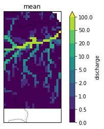
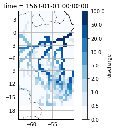
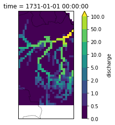
Discharge during the mega-floods
How did the flood-pulse look like for the two mega-floods and how did it build up? -> assess the spatial extent during the event and the temporal variability over the year.
Here, as a first, I show the spatial distribution of discharge during the mega-floods and during mean conditions.
In this notebook I have used the annual monthly maxima available through Zenodo. Then in notebook 1.2 I will look at the temporal distribution in the data Niko sent me, that contains all the months for the 2000 years. I will extract the years of the highest events and show how the simulated flood pulse looked like.
The highest flood occurs on 1568 (index 1567 in python). The second highest on 1731 (index 1730 in python).
For megaflood1 this corresponds to: Year: 2037 Start: 13 Ensemble: 13
And for megaflood2 this corresponds to: Year: 2035 Start: 14 Ensemble: 21
import matplotlib.ticker as mticker
# gl = ax.gridlines(crs=ccrs.PlateCarree(), draw_labels=True,
#                   linewidth=2, color='gray', alpha=0.5, linestyle='--')

levels = [0, 0.5, 1, 2, 5, 10, 20, 50, 100]

Amazon_discharge_flood1=Amazon_discharge.sel(time=megaflood1.time) / megaflood1.values.flatten() *100
Amazon_discharge_flood2=Amazon_discharge.sel(time=megaflood2.time) / megaflood2.values.flatten() *100
Amazon_discharge_mean=Amazon_discharge.mean(dim='time') / Amazon_timeseries.mean().values.flatten() *100
Amazon_timeseries.mean()
Amazon_discharge_mean
# Amazon_spatial.mean(dim='time') / meanflood * 100

map_proj = ccrs.Mercator()
# extent = [-85, -35, 15, -25]
extent = [-63, -50, 5, -20]

ax = plt.axes(projection=map_proj)
ax.set_extent(extent)
ax.coastlines(resolution='110m')
ax.add_feature(cartopy.feature.BORDERS, linestyle=':')
gl= ax.gridlines(draw_labels=True)
gl.xlabels_top = False
gl.ylabels_right = False
# gl.xlines = False
gl.xlocator = mticker.FixedLocator([-65,-60,-55,-50])
Amazon_discharge_flood1.plot(levels=levels,cmap=plt.cm.Blues,transform=ccrs.PlateCarree(), ax=ax)
plt.show()

ax2 = plt.axes(projection=map_proj)
ax2.set_extent(extent)
ax2.coastlines(resolution='110m')
ax2.add_feature(cartopy.feature.BORDERS, linestyle=':')
# ax.gridlines(draw_labels=True)
Amazon_discharge_flood2.plot(levels=levels,transform=ccrs.PlateCarree(), ax=ax2)
plt.show()

ax3 = plt.axes(projection=map_proj)
ax3.set_extent(extent)
ax3.coastlines(resolution='110m')
ax3.add_feature(cartopy.feature.BORDERS, linestyle=':')
# ax.gridlines(draw_labels=True)
Amazon_discharge_mean.plot(levels=levels,transform=ccrs.PlateCarree(), ax=ax3)
ax3.set_title('mean')
/home/tike/miniconda3/envs/exp/lib/python3.8/site-packages/xarray/core/nanops.py:142: RuntimeWarning: Mean of empty slice
  return np.nanmean(a, axis=axis, dtype=dtype)
- 349801.72
array(349801.72, dtype=float32)
- lat: 44
- lon: 70
- nan nan nan nan nan ... 0.04821367 0.2217864 0.02408495 1.7758697
array([[ nan, nan, nan, ..., nan, nan, nan], [ nan, nan, nan, ..., nan, nan, nan], [ nan, nan, nan, ..., nan, nan, nan], ..., [ nan, nan, nan, ..., 0.15629555, 0.02193377, 0.01489759], [ nan, nan, nan, ..., 0.04558183, 0.25920117, 2.057166 ], [ nan, nan, nan, ..., 0.2217864 , 0.02408495, 1.7758697 ]], dtype=float32) - lat(lat)float324.75 4.25 3.75 ... -16.25 -16.75
- long_name :
- latitude
- units :
- degrees_north
- standard_name :
- latitude
array([ 4.75, 4.25, 3.75, 3.25, 2.75, 2.25, 1.75, 1.25, 0.75, 0.25, -0.25, -0.75, -1.25, -1.75, -2.25, -2.75, -3.25, -3.75, -4.25, -4.75, -5.25, -5.75, -6.25, -6.75, -7.25, -7.75, -8.25, -8.75, -9.25, -9.75, -10.25, -10.75, -11.25, -11.75, -12.25, -12.75, -13.25, -13.75, -14.25, -14.75, -15.25, -15.75, -16.25, -16.75], dtype=float32) - lon(lon)float32-79.75 -79.25 ... -45.75 -45.25
- standard_name :
- longitude
- long_name :
- longitude
- units :
- degrees_east
array([-79.75, -79.25, -78.75, -78.25, -77.75, -77.25, -76.75, -76.25, -75.75,
       -75.25, -74.75, -74.25, -73.75, -73.25, -72.75, -72.25, -71.75, -71.25,
       -70.75, -70.25, -69.75, -69.25, -68.75, -68.25, -67.75, -67.25, -66.75,
       -66.25, -65.75, -65.25, -64.75, -64.25, -63.75, -63.25, -62.75, -62.25,
       -61.75, -61.25, -60.75, -60.25, -59.75, -59.25, -58.75, -58.25, -57.75,
       -57.25, -56.75, -56.25, -55.75, -55.25, -54.75, -54.25, -53.75, -53.25,
       -52.75, -52.25, -51.75, -51.25, -50.75, -50.25, -49.75, -49.25, -48.75,
       -48.25, -47.75, -47.25, -46.75, -46.25, -45.75, -45.25], dtype=float32)
<cartopy.mpl.feature_artist.FeatureArtist at 0x2b0f57d837f0>
<cartopy.mpl.feature_artist.FeatureArtist at 0x2b0f56c04d90>
<matplotlib.collections.QuadMesh at 0x2b0f57decac0>
<cartopy.mpl.feature_artist.FeatureArtist at 0x2b0f57f23f40>
<cartopy.mpl.feature_artist.FeatureArtist at 0x2b0f57e653d0>
<matplotlib.collections.QuadMesh at 0x2b0f57f2ec10>
<cartopy.mpl.feature_artist.FeatureArtist at 0x2b0f57fcc6a0>
<cartopy.mpl.feature_artist.FeatureArtist at 0x2b0f57f86430>
<matplotlib.collections.QuadMesh at 0x2b0f57fccd60>
Text(0.5, 1.0, 'mean')