Flood frequency curves for the Amazon
Load data
The data we use in this study consists of HYBAM observed streamflow records and simulated present climate streamflow simulations run by EC-EARTH and PCR-GLOBWB. The data are preprocessed in (Preprocessing streamflow records), selecting the annual maximum monthly streamflow.
Here we load the required packages and the data
library('UNSEEN')
library('dplyr')
library('ggplot2')
library('extRemes')
library('qmap')
library('moments')
Warning message:
“replacing previous import ‘vctrs::data_frame’ by ‘tibble::data_frame’ when loading ‘dplyr’”

Attaching package: ‘dplyr’


The following objects are masked from ‘package:stats’:

    filter, lag


The following objects are masked from ‘package:base’:

    intersect, setdiff, setequal, union


Loading required package: Lmoments

Loading required package: distillery


Attaching package: ‘extRemes’


The following objects are masked from ‘package:stats’:

    qqnorm, qqplot


Loading required package: fitdistrplus

Loading required package: MASS


Attaching package: ‘MASS’


The following object is masked from ‘package:dplyr’:

    select


Loading required package: survival
## The CABra observations, with a homogeneous period over all three Amazonian subcatchments of interest.
Observations_pooled_annual_df <- read.csv(file = '../Data/Observations_pooled_annual_df.csv')

# Obidos_record_annual_df_CABra <- read.csv(file ='../Data/Obidos_CABra_record_annual_df.csv')
# Xingu_record_annual_df_CABra <- read.csv(file ='../Data/Xingu_CABra_record_annual_df.csv')
# Tapajos_record_annual_df_CABra <- read.csv(file ='../Data/Tapajos_CABra_record_annual_df.csv')
We convert the streamflow to specific discharge to allow for a meaningful comparison between observations and simulations (and adjust for the difference in the catchment size). We obtain the catchment size from the CABra shiny app.
area_Obidos <- 4807564 * 1e6# in km2 -> m2. From GRDC data 4640300: https://www.compositerunoff.sr.unh.edu/html/Polygons/P3629000.html
area_Xingu <- 447711 * 1e6# in km2 -> m2.
area_Tapajos <- 459185 * 1e6# in km2 -> m2.
area_Amazon <- 5756000 * 1e6# in km2 -> m2. Obtained from model mask.
And we calculate the specific discharge for
Obidos + Tapajos + Xingu (Observed pooled)
the simulations at the Amazon mouth (UNSEEN)
The catchment areas of Obidos, Tapajos, and Xingu represent 99,3% of the catchment area within the model simulations and, hence, can be reasonably compared.
(area_Obidos + area_Xingu + area_Tapajos) / area_Amazon * 100
##Convert m3/s to mm/h -> divide by area (m3 to m) times 1000 (m to mm) and times 3600 (sec to hour)
## Monthly sum -> times 24 (hourly to daily) times 31 (days in July)
Observed_pooled <- ((Observations_pooled_annual_df$Streamflow) /
                         (area_Obidos + area_Xingu + area_Tapajos) * 1000 * 3600 * 24 #* 31
                         )

UNSEEN <- Amazon_annual_df$discharge / area_Amazon * 1000 * 3600 * 24 #* 31
We apply quantile mapping to adjust the annual maximum streamflow simulations to the observed record. We use the homogeneous observations and simulations for the Amazon outlet.
fit_qmap <- fitQmap(obs = Observed_pooled,
                    mod = UNSEEN,
                    method="QUANT", #method=c("RQUANT","QUANT","SSPLIN")
                    wet.day = FALSE)

UNSEEN_qmap_lin <- doQmap(x = UNSEEN,
                                 fobj = fit_qmap,
                                 type='linear')
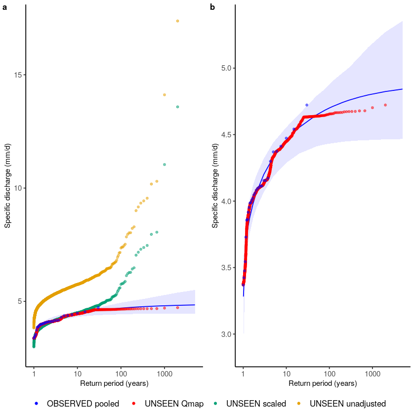
We then plot the empirical extreme value distributions for the observed record and the UNSEEN data.
## Load source code to plot extreme value distributions
source('src/evt_plot.r')
## For the legend we define the names and their corresponding colors here
cols <- c("UNSEEN unadjusted" = "#E69F00","UNSEEN scaled" = "#009E73","UNSEEN Qmap" = "red", "OBSERVED pooled" = "blue", "OBSERVED adjusted" = "black") ##  for  the legend

## And then plot
p1 <- ggplot() +
  geom_EVT_GEV(data = Observed_pooled,
               GEV_type = 'GEV',
               estimation_method = "MLE",
               CI_method = "boot",
               CI_significance = 0.05,
               transparency = 0.1,
               name = "OBSERVED pooled") +
  geom_EVT_empirical(UNSEEN, name = "UNSEEN unadjusted") +
  geom_EVT_empirical(UNSEEN * mean(Observed_pooled)/mean(UNSEEN), name = "UNSEEN scaled") + # scaling factor mean annual maxima
  geom_EVT_empirical(UNSEEN_qmap_lin, name = "UNSEEN Qmap") +
#   geom_EVT_empirical(Observed, name = "OBSERVED unadjusted") +
  geom_EVT_empirical(Observed_pooled, name = "OBSERVED pooled") +
scale_x_continuous(trans = "log10") +
  scale_colour_manual(name = "Data", values = cols) +
  scale_fill_manual(name = "GEV", values = cols) +
  theme_classic() +
  theme(
    legend.title = element_blank(),
    text = element_text(size = 9),
    axis.text = element_text(size = 9),
    legend.text = element_text(size = 10)
  ) +
  labs(y = "Specific discharge (mm/d)", x = "Return period (years)") +
  guides(fill = FALSE,
         color = guide_legend(override.aes = list(linetype = 0)))
Warning message in log(z):
“NaNs produced”
Warning message in log(z):
“NaNs produced”
Warning message in log(z):
“NaNs produced”
Warning message in log(z):
“NaNs produced”
Warning message in log(z):
“NaNs produced”
Warning message in log(z):
“NaNs produced”
Warning message in log(z):
“NaNs produced”
Warning message in log(z):
“NaNs produced”
Warning message in log(z):
“NaNs produced”
Warning message in log(z):
“NaNs produced”
Warning message in log(z):
“NaNs produced”
Warning message in log(z):
“NaNs produced”
Warning message in log(z):
“NaNs produced”
Warning message in log(z):
“NaNs produced”
Warning message in log(z):
“NaNs produced”
Warning message in log(z):
“NaNs produced”
Warning message in log(z):
“NaNs produced”
Warning message in log(z):
“NaNs produced”
Warning message in log(z):
“NaNs produced”
Warning message in log(z):
“NaNs produced”
Warning message in log(z):
“NaNs produced”
Warning message in log(z):
“NaNs produced”
Warning message in log(z):
“NaNs produced”
Warning message in log(z):
“NaNs produced”
Warning message in log(z):
“NaNs produced”
Warning message in log(z):
“NaNs produced”
Warning message in log(z):
“NaNs produced”
Warning message in log(z):
“NaNs produced”
Warning message in log(z):
“NaNs produced”
Warning message in log(z):
“NaNs produced”
## And for just obs and Qmap
p2 <- ggplot() +
  geom_EVT_GEV(data = Observed_pooled,
               GEV_type = 'GEV',
               estimation_method = "MLE",
               CI_method = "boot",
               CI_significance = 0.05,
               transparency = 0.1,
               name = "OBSERVED pooled") +
  geom_EVT_empirical(UNSEEN_qmap_lin, name = "UNSEEN Qmap") +
#   geom_EVT_empirical(Observed, name = "OBSERVED unadjusted") +
  geom_EVT_empirical(Observed_pooled, name = "OBSERVED pooled") +
  scale_x_continuous(trans = "log10") +
  scale_colour_manual(name = "Data", values = cols) +
  scale_fill_manual(name = "GEV", values = cols) +
  theme_classic() +
  theme(
    legend.title = element_blank(),
    text = element_text(size = 9),
    axis.text = element_text(size = 9),
    legend.text = element_text(size = 10)
  ) +
  labs(y = "Specific discharge (mm/d)", x = "Return period (years)") +
  guides(fill = FALSE,
         color = guide_legend(override.aes = list(linetype = 0)))
Warning message in log(z):
“NaNs produced”
Warning message in log(z):
“NaNs produced”
Warning message in log(z):
“NaNs produced”
Warning message in log(z):
“NaNs produced”
Warning message in log(z):
“NaNs produced”
Warning message in log(z):
“NaNs produced”
Warning message in log(z):
“NaNs produced”
Warning message in log(z):
“NaNs produced”
Warning message in log(z):
“NaNs produced”
Warning message in log(z):
“NaNs produced”
Warning message in log(z):
“NaNs produced”
Warning message in log(z):
“NaNs produced”
ggarrange(p1,p2,
          common.legend = TRUE,
          legend = "bottom",
          labels = c("a", "b"),
          font.label = list(size = 10, color = "black", face ="bold", family = NULL),
          # vjust = 0,
          ncol = 2, nrow = 1) #%>%
#   ggsave(filename = '../Graphs/Extreme_value_plot_corrections_obs_test.pdf',width =174,height = 75, units='mm',dpi=300) #174 for wide graphs
Testing bias corrections
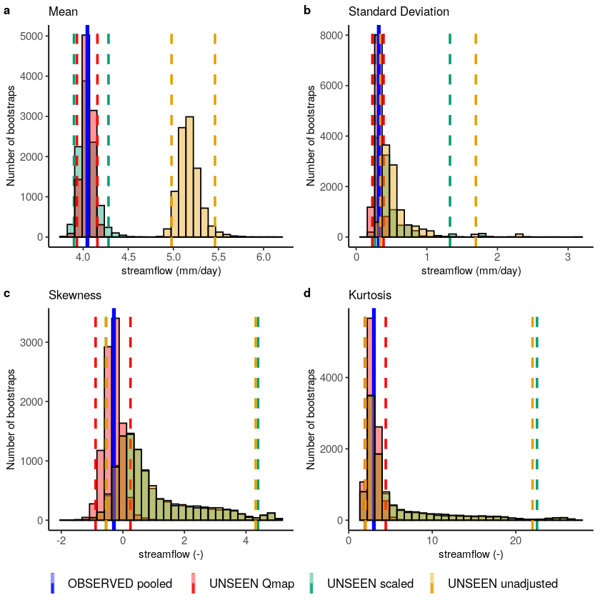
We test the consistency between the simulated and observed annual maximum specific discharge.
Fidelity_test_biascor(obs = Observed_pooled,
                      color_obs = "OBSERVED pooled",
                      ensemble = UNSEEN,
                      fill_ensemble = "UNSEEN unadjusted",
                      ensemble_cor1 = UNSEEN * mean(Observed_pooled)/mean(UNSEEN),
                      fill_ensemble_cor1 = "UNSEEN scaled",
                      ensemble_cor2 = UNSEEN_qmap_lin,
                      fill_ensemble_cor2 = "UNSEEN Qmap",
                      xlim_sd = c(NA,0.75),
                      xlim_kurt =c(NA,10),
                      cols = cols,
                      fontsize = 10
                      ) #%>%
#   ggsave(filename = '../Graphs/Fidelity_biascor_obs_test.pdf',width =174,height = 120, units='mm',dpi=300) #174 for wide graphs
Warning message:
“Removed 697 rows containing non-finite values (stat_bin).”
Warning message:
“Removed 1446 rows containing non-finite values (stat_bin).”
Warning message:
“Removed 1 rows containing missing values (geom_bar).”
Warning message:
“Removed 1 rows containing missing values (geom_vline).”
Warning message:
“Removed 1 rows containing missing values (geom_bar).”
Warning message:
“Removed 1 rows containing missing values (geom_bar).”
Warning message:
“Removed 1 rows containing missing values (geom_vline).”
Warning message:
“Removed 1580 rows containing non-finite values (stat_bin).”
Warning message:
“Removed 1582 rows containing non-finite values (stat_bin).”
Warning message:
“Removed 1 rows containing missing values (geom_bar).”
Warning message:
“Removed 1 rows containing missing values (geom_vline).”
Warning message:
“Removed 1 rows containing missing values (geom_bar).”
Warning message:
“Removed 1 rows containing missing values (geom_bar).”
Warning message:
“Removed 1 rows containing missing values (geom_vline).”
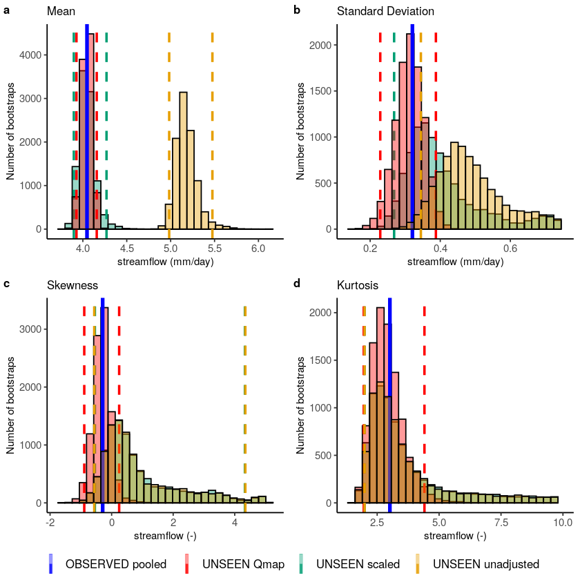
Fidelity_test_biascor(obs = Observed_pooled,
                      color_obs = "OBSERVED pooled",
                      ensemble = UNSEEN,
                      fill_ensemble = "UNSEEN unadjusted",
                      ensemble_cor1 = UNSEEN * mean(Observed_pooled)/mean(UNSEEN),
                      fill_ensemble_cor1 = "UNSEEN scaled",
                      ensemble_cor2 = UNSEEN_qmap_lin,
                      fill_ensemble_cor2 = "UNSEEN Qmap",
                      # xlim_sd = c(NA,1),
                      # xlim_kurt =c(NA,10),
                      cols = cols,
                      fontsize = 10
                      ) #%>%
#   ggsave(filename = '../Graphs/Fidelity_biascor_fullrange_obs_test.pdf',width =174,height = 120, units='mm',dpi=300) #174 for wide graphs